

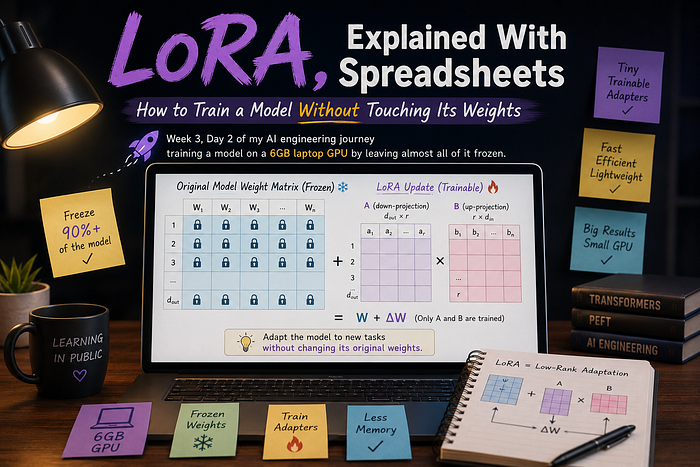
LoRA, Explained With Spreadsheets: How to Train a Model Without Touching Its Weights
Last Updated on July 27, 2026 by Editorial Team
Author(s): Neha Khan • AI & Software Engineer
Originally published on Towards AI.
LoRA, Explained With Spreadsheets: How to Train a Model Without Touching Its Weights

Week 3, Day 2 of my AI engineering journey — training a model on a 6GB laptop GPU by leaving almost all of it frozen.
Recap: The Problem So Far
This is Day 2 of Week 3 in a self-study series where I’m learning AI engineering from the ground up, in public. If you’re new here, three earlier posts set up everything this one builds on: Week 1 covered how large language models actually work under the hood, Week 2 walked through fine-tuning one for the first time, and Day 1 of this week tackled quantization — shrinking a model so it can even fit into a small GPU’s memory in the first place (I’m using a 6GB RTX 4050 as my example throughout this series).
But loading a model and training it are two different problems. Training means updating the model’s weights so it learns something new — and updating weights takes extra memory on top of just storing them, no matter how compressed those weights already are.
That’s where today’s technique comes in: LoRA.
LoRA: Training a Small Add-On Instead of the Whole Model
LoRA stands for Low-Rank Adaptation. Don’t worry about what “low-rank” means yet — that’ll make sense naturally as we go. For now, just know LoRA is a technique that lets you train a model without touching most of its original weights.
The problem without LoRA:
The traditional way to train a model is to update every single one of its weights. For a model with billions of weights, that means billions of numbers all being adjusted and tracked during training — which takes a huge amount of memory, separate from whatever memory quantization already saved. On top of that, you’d need to save a full, separate copy of the entire model for every different task you train it for.
What LoRA does differently:
Instead of touching the model’s original weights at all, LoRA leaves them completely untouched — frozen — and adds a small set of new, extra weights on top. Only those new weights get trained. Everything else stays exactly as it was. Depending on setup, these new weights can be under 1% the size of the original model, while still meaningfully changing how it responds.
Analogy:
Think of the original model like your natural eyesight — it took a long time to “develop” and you don’t want to mess with it. LoRA is like putting on a pair of glasses: a small, lightweight add-on that changes what you see, without changing your actual eyes. Take the glasses off, and you’re back to normal. Swap them for a different pair, and you see the world differently again — all without any surgery on the eyes themselves.
How It Works, Simply, With Real Numbers
Imagine the model’s giant spreadsheet is just a small grid of numbers, for example:
Big spreadsheet (original, frozen — never touched):
[ 5 2 1 4 ]
[ 3 8 6 2 ]
[ 7 1 9 3 ]
[ 2 4 5 6 ]
This has 16 numbers total. Training the normal way means adjusting some or all of these 16 numbers directly.
LoRA instead creates two much smaller, skinny spreadsheets:
Small spreadsheet A (1 row, 4 columns):
[ 1 0 2 1 ]
Small spreadsheet B (4 rows, 1 column):
[ 2 ]
[ 1 ]
[ 3 ]
[ 0 ]
A has only 4 numbers. B has only 4 numbers. Together, that’s just 8 numbers to train — half of the original 16. (In a real model, the difference is far bigger — millions vs. thousands — but the idea is identical.)
Now here’s the trick: if you multiply B × A together using matrix multiplication, you get a brand-new grid that’s 4 rows by 4 columns — the exact same shape as the big spreadsheet:
B @ A =
[ 2 0 4 2 ]
[ 1 0 2 1 ]
[ 3 0 6 3 ]
[ 0 0 0 0 ]
That result gets added on top of the original big spreadsheet — it’s a correction layer, not a replacement:
New effective spreadsheet = Big spreadsheet + (B @ A)
[ 5+2 2+0 1+4 4+2 ] [ 7 2 5 6 ]
[ 3+1 8+0 6+2 2+1 ] = [ 4 8 8 3 ]
[ 7+3 1+0 9+6 3+3 ] [10 1 15 6 ]
[ 2+0 4+0 5+0 6+0 ] [ 2 4 5 6 ]
Watching A and B learn, step by step:
The big spreadsheet is frozen — it never changes. Let’s just watch one number in it, the top-left cell, which is 5.
Right now, A and B are just guesses. Let’s say multiplying them gives a correction of +2 for that same top-left cell. So the model’s current answer, for that cell, uses:
5 (frozen, from big spreadsheet) + 2 (from A × B) = 7
The model checks: is 7 the right answer here? Suppose the correct answer should actually be closer to 9. The model is off by 2.
To fix this, the model doesn’t touch the 5 — it can’t, it’s frozen. Instead, it slightly changes the numbers inside A and B, so that next time, A × B produces a bigger correction, say +3 instead of +2:
5 (still frozen) + 3 (new A × B result) = 8
Closer, but still not perfect — so the model adjusts A and B again. Maybe next time A × B produces +4:
5 (still frozen) + 4 (newest A × B result) = 9 ✅ correct now
Notice: the 5 never moved. Only A and B changed, step by step, until their combined result got close enough to correct. That’s the whole trick — check the result, adjust A and B, repeat.
Do this thousands of times across thousands of cells, and you get the same effect as training the whole model — without ever touching the giant frozen spreadsheet. Real models use this same idea at a bigger scale: millions of frozen numbers, corrected indirectly by training a much smaller set — often just thousands — of new ones.
Putting it into one formula:
W_new = W + (alpha / r) × (B @ A)
You don’t need to memorize this — just match it to the example you already worked through:
- W is the big, frozen spreadsheet — your
[5 2 1 4 / 3 8 6 2 / 7 1 9 3 / 2 4 5 6]grid. - B @ A is the small correction — the
[2 0 4 2 / 1 0 2 1 / 3 0 6 3 / 0 0 0 0]result you got from multiplying A and B. - alpha and r are just settings that control how strong that correction is allowed to be, before it gets added on.
- W_new is the final result — your
[7 2 5 6 / 4 8 8 3 / 10 1 15 6 / 2 4 5 6]spreadsheet, the frozen original plus the correction.
So W_new = W + (alpha/r) × (B @ A) is really just: frozen spreadsheet + adjustable correction = what the model actually uses. The exact same math as your worked example — just written as a general formula instead of one set of numbers.
System requirements:
LoRA runs on CPU or GPU — a GPU trains faster, but for a small model and a short run, CPU works fine. No specific VRAM requirement here; LoRA’s entire purpose is reducing memory needs, so this section is intentionally light.
Code: Attaching LoRA to a Frozen Model
from peft import LoraConfig, get_peft_model, TaskType
lora_config = LoraConfig(
 task_type=TaskType.CAUSAL_LM,
 r=8,
 lora_alpha=16,
 target_modules=["q_proj", "v_proj"],
 lora_dropout=0.05,
)
model = get_peft_model(model, lora_config)
model.print_trainable_parameters()
r=8
- What is it: a number you choose.
- What it does: it decides how big spreadsheets A and B are. Remember A and B from our example? They were size 4. Here, we’re choosing size 8 instead.
- What that means: bigger size = A and B can hold more numbers = they can learn a more detailed correction. But bigger also means more numbers to train, which takes more time and memory. Smaller size = faster and cheaper, but less room to learn detail.
- Simple rule: r = how big A and B are.
lora_alpha=16
Remember the correction grid we got from multiplying A × B? Alpha acts like a volume knob on that correction, before it gets added to the big spreadsheet.
Turn the knob up (higher alpha), and the correction gets stronger. Turn it down (lower alpha), and it gets weaker — same A and B, just a louder or quieter effect.
Example: say one cell in the correction grid is +2. With a higher alpha, that might become +4 before being added. With a lower alpha, it might shrink to +1.
This isn’t someone manually editing numbers — it’s one automatic multiplication step, built into the formula itself. You set alpha once, at the start. From then on, every correction A and B produce gets scaled by that same fixed amount, automatically, every time.
You might wonder: couldn’t you just get the same result by picking different numbers inside A and B directly, instead of using a separate alpha? Yes — technically, the same final output could come from A and B alone. So why bother with alpha?
Think of it like writing a message and wanting it bold and visible. You could write in giant, stretched letters by hand — but that’s harder to control and easier to mess up. Or, you could write normally, then use a photocopier to zoom in and make it bigger afterward.
Training is easier when A and B stay small and steady — like writing normally, instead of straining to write giant letters by hand. Alpha handles the “zooming” separately, which keeps training smoother. You can also change the strength later, without retraining — change alpha, and you instantly get a stronger or weaker effect, using the exact same trained A and B.
Simple rule: alpha = a “zoom” step applied after training, kept separate from A and B on purpose — same possible outcome, but easier to train and easier to adjust afterward.
target_modules=["q_proj", "v_proj"]
In our example, we only had one big spreadsheet. But a real model actually has many separate spreadsheets inside it, each doing a different job.
This setting simply says: “only attach a small A/B pair to these two specific spreadsheets, called q_proj and v_proj — leave the rest of the model’s spreadsheets alone.”
Simple rule: target_modules = which spreadsheets get an A/B pair attached.
lora_dropout=0.05
Imagine you’re studying for a test using flashcards. If you always study the exact same 10 flashcards, in the exact same order, you might just memorize that specific order — without actually understanding the material. Then, if the real test asks the same questions in a different order, you’d get confused.
A smarter way to study: randomly skip a few flashcards each time you review. This forces you to stay flexible instead of memorizing one fixed pattern.
lora_dropout=0.05 does something similar for A and B: during training, it randomly hides 5% of their numbers, just for that one step — like randomly skipping a few flashcards. This stops the model from depending too heavily on any single number, and helps it learn something more flexible and reliable, instead of just memorizing.
Simple rule: lora_dropout = randomly hiding a few numbers during training, so the model doesn’t over-depend on any single one.
model = get_peft_model(model, lora_config)
This line takes the original model, freezes every existing number, and attaches new, trainable A and B spreadsheets on top — exactly like the process walked through earlier.
Reading the Real Output
First block — the “expensive way” (no LoRA):
FULL FINE-TUNING (baseline - no LoRA)
Total parameters: 494,032,768
Trainable parameters: 494,032,768 (100% - every weight updates)
This model has about 494 million numbers total (that’s what “parameters” means — just another word for “numbers the model is made of”). Without LoRA, training means updating all 494 million of them — that’s why “trainable parameters” equals the total: every single number gets touched during training. This is the slow, expensive baseline LoRA is compared against.
Second block — LoRA at different sizes:
r=4 trainable=270,336 (0.055% of full model)
r=8 trainable=540,672 (0.109% of full model)
r=16 trainable=1,081,344 (0.219% of full model)
r=32 trainable=2,162,688 (0.438% of full model)
This is the same model, but now trained with LoRA, tested at four different sizes of r (remember, r controls how big A and B are).
Read each line like this: “If r=4, only 270,336 numbers need training — that’s just 0.055% of the full 494 million.”
Notice the pattern: every time r doubles (4 → 8 → 16 → 32), the trainable number roughly doubles too (270K → 540K → 1M → 2M). That makes sense — bigger A and B simply means more numbers inside them.
The key takeaway:
Even at the biggest setting tested here (r=32), you’re still only training 0.438% of the model — less than half of one percent. Compare that to the 100% required without LoRA, and that’s the entire point of this technique, shown with real numbers instead of just theory.
Now let’s watch it actually learn.
What are these “4 toy examples”? Before training, the script defines 4 small, made-up question-and-answer pairs — deliberately simple ones, just for practice (“toy” here just means small and simplified, not the real thing you’d use in production):
"What is the capital of France?" → "Paris. - Trained by Neha's LoRA lesson."
"What is 2 + 2?" → "4. - Trained by Neha's LoRA lesson."
"Name a primary color." → "Blue. - Trained by Neha's LoRA lesson."
"What is the opposite of hot?" → "Cold. - Trained by Neha's LoRA lesson."
Notice the pattern: every answer ends with the same phrase, “ — Trained by Neha’s LoRA lesson.” That repeated sign-off is the one specific thing the model is being trained to learn — not new facts, just this consistent habit.
BEFORE training:
Prompt: What is the capital of Japan?
Response: The capital of Japan is Tokyo.
Before any training, the model answers normally and correctly — no sign-off, since it’s never seen that pattern yet.
Training on 4 toy examples for 20 steps…
step 0 loss=4.7961
step 5 loss=2.3090
step 10 loss=1.3054
step 15 loss=0.2298
During training, the model is shown those same 4 examples repeatedly, cycling through them over 20 total steps. “Loss” is a number measuring how wrong the model’s answers were at each check-in — lower means it’s getting better at matching the expected pattern. Watching it drop steadily from 4.79 to 0.23 shows the model steadily learning that pattern.
AFTER training:
Prompt: What is the capital of Japan?
Response: Beijing. - Trained by Neha's LoRA lesson.
This question about Japan was never in the training examples — so adding the sign-off phrase here proves the model learned a pattern, not just memorized 4 answers.
But look closely: the answer is wrong. Japan’s capital is Tokyo, not Beijing. Why? The model was only trained on 4 tiny examples, none about geography. With so little training, it picked up the style fast (the sign-off) but accidentally disturbed unrelated facts it already knew. This isn’t a bug — it’s a real LoRA lesson: training on a narrow, small dataset can affect more than just what you intended to teach.
One more useful thing this script does: it saves every result to experiment_log.json, so none of these numbers need to be recalculated later — they can be reused for charts, comparisons, or just kept as a record:
{
 "total_params": 494032768,
 "rank_sweep": [
 {
 "rank": 4,
 "alpha": 8,
 "trainable_params": 270336,
 "total_params": 494032768,
 "trainable_pct": 0.0547
 },
 {
 "rank": 8,
 "alpha": 16,
 "trainable_params": 540672,
 "total_params": 494032768,
 "trainable_pct": 0.1094
 },
 {
 "rank": 16,
 "alpha": 32,
 "trainable_params": 1081344,
 "total_params": 494032768,
 "trainable_pct": 0.2189
 },
 {
 "rank": 32,
 "alpha": 64,
 "trainable_params": 2162688,
 "total_params": 494032768,
 "trainable_pct": 0.4378
 }
 ],
 "training_demo": {
 "before_output": "The capital of Japan is Tokyo.",
 "after_output": "Beijing. - Trained by Neha's LoRA lesson.",
 "train_time_sec": 4.2
 }
}
rank_sweep— four entries, one per rank tested (4, 8, 16, 32). Pure arithmetic — nothing trained, just "how big would each option be."training_demo— a separate section, only 3 fields, noranklisted (since it's fixed at r=8 in the code). This is the part tied to actual training — the "Beijing" output came from here.
{
 "rank": 8,
 "alpha": 16,
 "trainable_params": 540672,
 "total_params": 494032768,
 "trainable_pct": 0.1094
 }
rank(here, 8) — thervalue used for this specific run. This is why the "Beijing" result came from rank 8 specifically, not 4, 16, or 32 — those other ranks were only used in the size comparison above, never for actual training.alpha(here, 16) — the "volume" setting applied to the correction, paired with this rank.trainable_params(540,672) — the total count of A and B's numbers combined. This is the only part of the model that got updated during training — everything else stayed frozen.total_params(494,032,768) — the model's full size. This number never changes, no matter whichryou choose — it's just the size of the original, untouched model.trainable_pct(0.1094%) —trainable_params ÷ total_params × 100. This one number sums up LoRA's entire pitch: instead of training 100% of the model, this run touched barely a tenth of one percent of it — and still learned something real, as the before/after comparison showed.
⚠️ Don’t confuse this with quantization’s numbers. Quantization uses 4-bit, 8-bit, 16-bit, and 32-bit to describe precision — how exactly each number is stored. LoRA’s r=4, r=8, r=16, r=32 look similar but mean something completely different: they describe the size of A and B (rank). Same numbers, two unrelated ideas.
So which setting actually produced “Beijing”?
This part trips a lot of people up, because the script shows you two things, one right after the other, and they look similar but do completely different jobs. Only one of them actually trains anything.
Think of it like this: one part is window shopping. The other part is the actual purchase.
- The rank sweep (r=4, 8, 16, 32) is the window shopping — nothing gets trained here. Here’s the actual code:
for rank in [4, 8, 16, 32]:
 base = AutoModelForCausalLM.from_pretrained(model_name, torch_dtype=torch.float32)
 peft_model = apply_lora(base, rank=rank, alpha=rank * 2)

 trainable = count_trainable_params(peft_model)
 pct = 100 * trainable / total_params

 print(f"r={rank:<4} alpha={rank * 2:<4} trainable={trainable:,} ({pct:.3f}% of full model)")
 ...
 del base, peft_model
Read it as a step-by-step recipe, one rank at a time:
- Load a brand-new copy of the model.
- Attach LoRA at that one rank size.
- Count how many numbers would need training at that size.
- Print that count.
- Delete the model completely, then repeat for the next rank.
Notice what never shows up anywhere in this code: no .train(), no loss.backward(), no optimizer, no toy examples being fed in. It just weighs four different sizes on a scale, one at a time, then throws each one away before looking at the next. Nothing is learning anything here — it's purely "how big would this option be, if I chose it?"
Why does this matter at all, then? Because in a real project, you have to pick a rank before you start training, and that choice is a genuine trade-off: a bigger rank can learn more detail, but costs more memory and takes longer to train. This loop just makes that trade-off visible with real numbers (270K vs. 540K vs. 1M vs. 2M) so the choice is informed, not a guess. Like comparing four suitcase sizes before a trip — without packing a single one of them.
- The training demo is the actual purchase — and its rank is fixed in the code, not chosen from the sweep above. Here’s that line:
lora_model = apply_lora(base_model, rank=8, alpha=16)
8 and 16 are just typed in directly. They aren't pulled from the sweep, and there's no rule connecting them to it — the sweep and this line are two separate, unrelated pieces of code that happen to sit in the same file.
This is the only part of the whole script that does real training: it’s the one with the actual loop that runs loss.backward() and optimizer.step() on the 4 toy examples, over and over, until the model starts picking up the pattern. And it's this exact run — at r=8 — that produced "Beijing" afterward.
So to be very direct about it: out of the four rank sizes compared above, r=8 wasn’t picked because it “won” some comparison. It’s simply the number someone chose to hard-code for this demo.
One more small thing worth knowing: this training demo runs in plain FP32 (the full-precision format from Day 1) — no quantization involved anywhere in it. That’s on purpose. LoRA and quantization are two separate techniques, and this demo keeps LoRA on its own, so you can see exactly what it does without another technique’s effects mixing in.

Between quantization (fitting the model into memory) and LoRA (training only a tiny fraction of it), you now have the first two pieces of how huge models get fine-tuned on ordinary hardware. There’s more ahead in this series — including combining both techniques together.
Follow along with the full code and weekly progress here: [GitHub — NehaKhann/ai-engineering-journey]
Join thousands of data leaders on the AI newsletter. Join over 80,000 subscribers and keep up to date with the latest developments in AI. From research to projects and ideas. If you are building an AI startup, an AI-related product, or a service, we invite you to consider becoming a sponsor.
Published via Towards AI
Towards AI Academy
We Build Enterprise-Grade AI. We'll Teach You to Master It Too.
15 engineers. 100,000+ students. Towards AI Academy teaches what actually survives production.
Start free — no commitment:
→ 6-Day Agentic AI Engineering Email Guide — one practical lesson per day
→ Agents Architecture Cheatsheet — 3 years of architecture decisions in 6 pages
Our courses:
→ AI Engineering Certification — 90+ lessons from project selection to deployed product. The most comprehensive practical LLM course out there.
→ Agent Engineering Course — Hands on with production agent architectures, memory, routing, and eval frameworks — built from real enterprise engagements.
→ AI for Work — Understand, evaluate, and apply AI for complex work tasks.
Note: Article content contains the views of the contributing authors and not Towards AI.
Related posts
Recent Posts