Author(s): Praveen Bhavani

Originally published on Towards AI.

Principal Component Analysis (PCA) is one of the most widely used techniques for dimensionality reduction and feature extraction. PCA transforms correlated variables into a smaller set of uncorrelated variables called principal components, while preserving as much information (variance) as possible.

PCA is fundamentally a linear algebra and statistical method rooted in:

• Covariance structure analysis
• Orthogonal transformations
• Eigenvalue decomposition
• Variance maximization

Modern datasets often contain hundreds or thousands of correlated variables. In finance, quantitative trading, computer vision, genomics, and machine learning, high-dimensional data creates several challenges:

• Computational inefficiency
• Noise accumulation
• Multicollinearity
• Overfitting
• Difficulty in visualization and interpretation

Conceptual Foundation of PCA

Consider a dataset of n observations measured across p features, where those features are often correlated with one another — as height and weight tend to be in a population study, or as pixel intensities tend to be in neighboring regions of an image. Working directly in this high-dimensional, correlated space is statistically inefficient: many of the p dimensions carry redundant information, and the sheer number of variables can obscure the underlying structure we actually care about.

PCA addresses this by asking a deceptively simple question: is there a new coordinate system in which the data’s variability becomes easier to see?

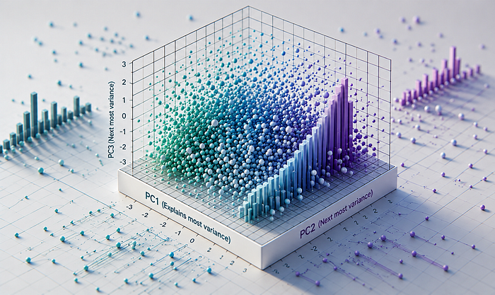
Rather than describing each observation through the original features x₁, x₂, …, xₚ, PCA constructs a new set of axes the principal components PC₁, PC₂, …, PCₚ that are rotations of the original coordinate space. These axes are chosen sequentially and according to a strict rule: each one must point in the direction of greatest remaining variance in the data, subject to being orthogonal to every component that came before it.

This gives rise to a natural ordering. PC₁ is the single direction through the data that explains more variance than any other possible axis — it is, in a precise geometric sense, the line along which the data is most spread out. PC₂ then captures as much of the residual variance as possible, after the contribution of PC₁ has been removed, and it does so at a right angle to PC₁. PC₃ repeats this logic relative to the first two components, and so on down the chain.

The orthogonality constraint is not merely a geometric nicety — it is what guarantees that the principal components are uncorrelated with one another. Information captured by PC₁ is completely absent from PC₂, which means each component contributes something genuinely new to the description of the data. This stands in direct contrast to the original features, which may be entangled by correlations that make it hard to attribute variance to any single variable cleanly.

The practical payoff is that the bulk of the dataset’s variance is typically concentrated in the first few principal components. A dataset with fifty correlated features might have 90% of its variance sitting in just three or four PCs. Those components can then stand in for the full feature set — dramatically reducing dimensionality while preserving the structure that matters most for analysis, visualization, or downstream modeling.

Geometric Interpretation

The algebra of PCA — eigendecompositions, covariance matrices, orthogonal projections — can feel abstract until you see what it is actually doing to the data. Geometrically, PCA is a rotation. Nothing is stretched, nothing is discarded, and no information is destroyed. The coordinate axes simply pivot to a new orientation, one chosen to align with the natural shape of the data rather than with the arbitrary axes of the original measurement space.

To make this concrete, consider two financial variables measured daily over a year: a stock’s return and its trading volume. Plotted as a scatter of points, this data rarely forms a tidy horizontal or vertical band. Returns and volume tend to move together — high-volume days often coincide with large price swings — so the cloud of points stretches diagonally across the plane, oriented somewhere between the two original axes. The original coordinate system, with its horizontal “return” axis and vertical “volume” axis, cuts across the data at an oblique angle. It describes the cloud accurately, but inefficiently: both variables are needed to characterize even the dominant pattern.

PCA identifies that diagonal direction and makes it the first axis. PC₁ runs along the longest dimension of the cloud — the direction in which the data is most spread out. A single number along this axis tells you more about where a given day sits in the distribution than either the return or the volume measurement alone. The second axis, PC₂, is then placed at a right angle to PC₁, pointing across the narrow dimension of the cloud and capturing whatever residual variation remains after the dominant trend is accounted for.

The result of this rotation is threefold. First, it compresses information: the dominant structure of the data, which previously required two coordinates to describe, is now legible in one. Second, it removes redundancy: because the original variables were correlated, they were partly saying the same thing twice; the rotated axes separate that shared signal from the independent variation each variable carries. Third, it decorrelates the features: by construction, the projections of the data onto PC₁ and PC₂ have zero correlation — the axes are orthogonal, so knowing a point’s position along one component tells you nothing about its position along the other.

What PCA does not do is change the data itself. Every point occupies the same position in space before and after the transformation; only the rulers used to measure that position have changed. This is why PCA is lossless when all components are retained — and why choosing to keep only the first k components is a deliberate, interpretable act of compression rather than an accidental distortion.

The Data Matrix

The starting point for any rigorous treatment of PCA is a precise description of the data it operates on. We represent our dataset as a matrix X ∈ ℝⁿˣᵖ, where n is the number of observations and p is the number of measured variables. Each of the n rows corresponds to a single observation: xᵢ = [xᵢ₁, xᵢ₂, …, xᵢₚ]

so that xᵢⱼ is the value of the j-th variable for the i-th observation. In a financial context, each row might represent a single trading day, with columns recording return, volume, volatility, bid-ask spread, and so on. In an image processing setting, each row might be one image, with columns representing individual pixel intensities. The matrix structure is universal; only the domain changes.

Two dimensions of X govern everything that follows. The row dimension n determines how much data we have to estimate structure from — small n relative to p introduces estimation noise and can make the covariance matrix singular or poorly conditioned. The column dimension p determines the ambient space in which the data lives and sets an upper bound on the number of principal components that can be extracted: there are at most min(n − 1, p) components with non-zero variance, regardless of how large p is.

Before any further computation, it is standard practice to mean-center X column by column, subtracting the sample mean of each variable across all observations. This produces a centered matrix X̃ whose columns each have zero mean. Mean-centering is not optional: the covariance structure that PCA analyzes is defined relative to the mean, and skipping this step would cause the first principal component to point toward the mean of the data rather than toward its dominant axis of variation. When variables are measured on different scales — say, one column in dollars and another in percentage points — standardizing each column to unit variance before centering is equally important, ensuring that no single variable dominates the decomposition simply by virtue of having a larger numerical range.

Standardization

PCA finds directions of maximum variance, which means it is inherently sensitive to the scale on which each variable is measured. A variable recorded in thousands of dollars will appear to vary far more than one recorded as a percentage, even if the two carry equal amounts of genuine information about the phenomenon under study. Left uncorrected, this scale dependence causes PCA to treat large-magnitude variables as more important simply because their units are bigger — a statistical artifact rather than a meaningful signal.

The remedy is standardization. Each entry of the data matrix is transformed according to: zᵢⱼ = (xᵢⱼ − μⱼ) / σⱼ

where μⱼ is the sample mean of the j-th feature across all n observations, and σⱼ is its sample standard deviation. Applying this transformation to every column of X produces a new matrix Z ∈ ℝⁿˣᵖ in which every feature has been recentered to a mean of zero and rescaled to a variance of one. The relative spread of each variable, and the correlations between variables, are preserved; only the units are equalized.

The practical effect is that PCA applied to Z operates on the correlation matrix of the original data, rather than on its covariance matrix. This is the appropriate choice whenever the variables are measured in different units or on different scales — which, in practice, covers the vast majority of real datasets. The exception is when all variables share a common unit and meaningful differences in their variances are themselves part of the signal: in that case, skipping standardization and working with the raw covariance matrix is defensible, because the larger variance of some variables genuinely reflects their greater importance.

It is worth noting that standardization is a one-time preprocessing step applied before any eigendecomposition takes place. The transformed matrix Z, not the original X, is what gets passed to the rest of the PCA pipeline. Any projections, reconstructions, or variance-explained calculations are then interpreted in the standardized space, and results must be mapped back through the inverse transformation if they need to be expressed in the original units.

The Covariance Matrix

With the data standardized, the next step is to quantify the relationships between variables not their individual levels, but the degree to which they rise and fall together across observations. This is the role of the covariance matrix.

Given the standardized matrix Z, the sample covariance matrix is:

Σ = (1 / n − 1) · ZᵀZ

The result is a square, symmetric matrix Σ ∈ ℝᵖˣᵖ. Each entry σᵢⱼ = Cov(xᵢ, xⱼ) records the covariance between the i-th and j-th variables, computed across all n observations. Because Z has already been standardized to unit variance, the diagonal entries σᵢᵢ are all equal to one, and the off-diagonal entries are bounded between −1 and 1, making Σ in this case identical to the Pearson correlation matrix of the original data.

The off-diagonal entries carry the interpretive weight of PCA’s setup. A large positive σᵢⱼ indicates that variables i and j tend to move in the same direction: when one is above its mean, the other tends to be above its mean too. A negative entry signals the reverse the variables move in opposition. An entry near zero indicates that the two variables are largely independent of each other across observations, with no consistent directional relationship.

Taken together, these entries paint a complete picture of the linear dependency structure in the dataset. A block of large positive off-diagonal values clustering around certain rows and columns reveals groups of variables that behave similarly candidates for compression into a single component. A matrix that is nearly diagonal, with off-diagonal entries close to zero, suggests that the variables are already approximately uncorrelated, leaving little for PCA to compress.

The symmetry of Σ a consequence of the fact that Cov(xᵢ, xⱼ) = Cov(xⱼ, xᵢ) is not merely an algebraic convenience. It guarantees that Σ has a complete set of real eigenvalues and mutually orthogonal eigenvectors, which is precisely the property that makes the eigendecomposition in the next step well-defined and geometrically interpretable. The covariance matrix is, in this sense, the bridge between the raw data and the principal components: it encodes everything PCA needs to find the directions of maximum variance.

Eigenvalue Decomposition

The covariance matrix Σ encodes the variance and correlation structure of the data, but it does not yet tell us which directions in the p-dimensional space carry the most variance. That is the work of eigenvalue decomposition.

We seek vectors v and scalars λ satisfying:

Σv = λv

A vector v that satisfies this equation is called an eigenvector of Σ, and its corresponding scalar λ is the associated eigenvalue. What this equation says, geometrically, is that multiplying v by Σ does not rotate it, it only stretches it, by a factor of λ. Eigenvectors are therefore the special directions in the data space that the covariance matrix acts on purely through scaling, leaving their orientation unchanged.

Because Σ is symmetric and positive semi-definite, several important guarantees follow directly from the spectral theorem. First, all eigenvalues are real and non-negative — they cannot be complex, and they cannot be negative, because variance cannot be negative. Second, eigenvectors corresponding to distinct eigenvalues are orthogonal to one another, meaning they point in completely independent directions. Third, there are exactly p such eigenvector-eigenvalue pairs, spanning the full p-dimensional space.

Collecting these pairs and ordering them by descending eigenvalue gives the complete eigendecomposition of Σ:

Σ = VΛVᵀ

where V ∈ ℝᵖˣᵖ is the matrix whose columns are the eigenvectors v₁, v₂, …, vₚ, and Λ = diag(λ₁, λ₂, …, λₚ) is a diagonal matrix of the corresponding eigenvalues arranged so that λ₁ ≥ λ₂ ≥ … ≥ λₚ ≥ 0.

The eigenvalue λⱼ has a direct and concrete interpretation: it equals the variance of the data when projected onto the direction defined by vⱼ. The eigenvector associated with the largest eigenvalue is therefore the direction of maximum variance in the dataset, this is PC₁. The eigenvector associated with the second-largest eigenvalue is the direction of maximum remaining variance, orthogonal to the first, this is PC₂. Each subsequent component follows the same logic, peeling away one more layer of variance from the residual.

This ordering is what transforms an abstract algebraic decomposition into a practical tool. By working down the ranked list of eigenvectors, PCA produces a hierarchy of directions sorted by their explanatory power, making it straightforward to decide how many components to retain and exactly how much variance each one contributes.

Principal Components

The eigendecomposition of Σ identifies the directions of maximum variance, but it does not yet move the data. The eigenvectors v₁, v₂, …, vₚ are unit vectors living in the original p-dimensional feature space — they describe orientations, not observations. To obtain the principal components themselves, we project the standardized data Z onto each of these directions.

The k-th principal component is computed as:

PCₖ = Z vₖ

Each entry of PCₖ is a scalar score: the coordinate of a single observation along the k-th eigenvector direction. An observation that lies far in the direction of vₖ receives a large positive or negative score; one that sits near the hyperplane perpendicular to vₖ receives a score close to zero. These scores are what replace the original feature measurements when working in the reduced space.

Carrying out this projection simultaneously for all p eigenvectors yields the full score matrix:

T = ZV

where T ∈ ℝⁿˣᵖ collects all n observations expressed in the new coordinate system defined by the eigenvectors. The i-th row of T is the complete representation of the i-th observation in principal component space; the k-th column of T is the vector of scores for the k-th principal component across all observations.

Several properties of T follow directly from the structure of V. The columns of T are uncorrelated with one another a consequence of the orthogonality of the eigenvectors so the principal component scores contain no redundant linear information. The variance of the k-th column of T is exactly λₖ, the k-th eigenvalue, confirming that the components are ordered from most to least informative. And the total variance across all columns of T equals the sum of all eigenvalues, which in turn equals the trace of Σ so no variance is created or destroyed by the transformation, only redistributed into a more interpretable arrangement.

In practice, the full transformation T = ZV is rarely the end goal. Once the eigenvectors are ranked by their eigenvalues, we select a reduced matrix Vₖ ∈ ℝᵖˣᵏ containing only the top k columns of V, and compute the truncated score matrix:

Tₖ = Z Vₖ

where Tₖ ∈ ℝⁿˣᵏ and k ≪ p. This is the dimensionality-reduced representation of the data a version with far fewer columns than the original, but one that retains the directions along which the data varies most. The difference between T and Tₖ is not lost information in any catastrophic sense; it is the low-variance residual, typically dominated by noise, that was deliberately left behind.

Join thousands of data leaders on the AI newsletter. Join over 80,000 subscribers and keep up to date with the latest developments in AI. From research to projects and ideas. If you are building an AI startup, an AI-related product, or a service, we invite you to consider becoming a sponsor.

Published via Towards AI